

How We Did Entity Resolution With a Vector DB and Argon


Key Takeaways
- VectorAI DB blocks each record to its 10 nearest neighbors, cutting Abt-Buy from 1,180,452 possible pairs to 10,810 while keeping 99% of true matches.
- A similarity threshold settles the clear-cut pairs, and Gemini 4 Argon reviews only the uncertain 13.2% band, returning a match decision with a one-sentence reason.
- The pipeline raises F1 from 0.813 to 0.915 and precision to 0.998 on Abt-Buy, at about $0.76 per 1,000 records.
- The Argon pass pays off when the band holds most of the threshold’s errors and Argon is at least about 10 points more accurate on those pairs.
- VectorAI DB and the embedding model run on your own infrastructure, so only the uncertain band leaves your network.
Somewhere in your customer, supplier, or product table, the same thing is listed twice. In the Abt-Buy benchmark, one catalog calls a TV “Sharp AQUOS 37′ Black LCD HDTV – LC37D64U” and the other calls it “Sharp AQUOS LC-37D64U 37′ LCD TV”. Finding pairs like these is entity resolution, and it gets hard fast. Checking every record against every other one means about 500 billion comparisons for a million rows. Similarity scores also fail on the close calls. The same catalog sells an LC37D44U, one character off and a different TV, and our embedding model scored it higher than the right one.

So we split the work. VectorAI DB narrows each record to its 10 nearest neighbors, which cut Abt-Buy from 1,180,452 possible pairs to 10,810 and kept 99% of the true matches. A similarity threshold settles the clear-cut calls. The uncertain 13.2% go to Gemini 4 Argon, a Google Gemini model that reads both records and returns a match or no-match with a one-sentence reason. We chose it for this experiment because it returns JSON that fits a schema, lets you cap how much it thinks, and can read the part number that the embedding blurs.
The threshold alone reached an F1 score of 0.813 (F1 balances precision and recall). With Argon on the uncertain pairs, F1 rose to 0.915 and precision to 0.998, for $0.76 per 1,000 records in the test split. In this article, you’ll build that pipeline step by step. You’ll learn how to block records with a filtered nearest-neighbor search in VectorAI DB and pick K from reduction ratio and pair completeness. You’ll also set the threshold band from your own data and test whether the Argon pass pays off before you spend money on it.
TL;DR
- Blocking: VectorAI DB kept 10,810 of the 1,180,452 possible Abt-Buy pairs, removing 99.08%, and kept 99.0% of the true matches.
- Threshold only: F1 0.813.
- With Argon on the uncertain band: F1 0.915, precision 0.998.
- Sent to Argon: 13.2% of candidate pairs, 1,001 of 7,570 on the test split.
- Cost: $1.41 at OpenRouter’s charges, or $0.76 per 1,000 records in the test split (757 Abt records plus all 1,092 Buy records).
- When it pays: When the band holds most of the threshold’s errors and Argon decides band pairs clearly better than the threshold. In our band-width tests, the slice where Argon led the threshold by 12 points bought 1.5 F1 points; slices where it led by about 1 point bought almost nothing.
Prerequisites
- Docker with the Compose plugin.
- uv, the Python package manager, which installs a compatible Python for you. The install command is below this list.
- Ollama, to run the embedding model locally.
- A Gemini 4 Argon key: an OpenRouter key with a few dollars of credit, or a Google AI Studio or Google Cloud key with billing turned on. Argon has no free tier; the Abt-Buy run cost $1.41.
- VectorAI DB, with no separate install: Step 1 runs Community Edition in Docker. Each benchmark fits under its 5,000-vector cap, one at a time.
- About 3 GB of free disk for the database image and the embedding model. Everything runs on a CPU; no GPU is needed.
Install uv if you don’t have it
# macOS or Linux
curl -LsSf https://astral.sh/uv/install.sh | sh

# Windows (PowerShell)
irm https://astral.sh/uv/install.ps1 | iex
All code is in the companion repo, and Step 1 clones it. In a hurry? Follow Steps 1 to 3, then skip to Step 8.
What You are Building
Entity resolution, also called record linkage or entity matching, runs in three steps. Blocking cuts the pairs down to candidates. Comparison scores each candidate, often with fuzzy matching on names and fields. Matching makes the final call. This build gives each step its own tool:
- VectorAI DB does the blocking. For each record, it returns the nearest neighbors from the other table- the records whose embeddings are closest- so the pipeline scores 10 candidates per record instead of every possible pair.
- EmbeddingGemma, run locally through Ollama, turns each record into a 768-dimensional vector.
- A similarity threshold auto-matches confident pairs and rejects clear non-matches.
- Gemini 4 Argon decides the uncertain band in between and gives a one-sentence reason.
resolve.pyconnects them and scores the results against the benchmark’s known matches.
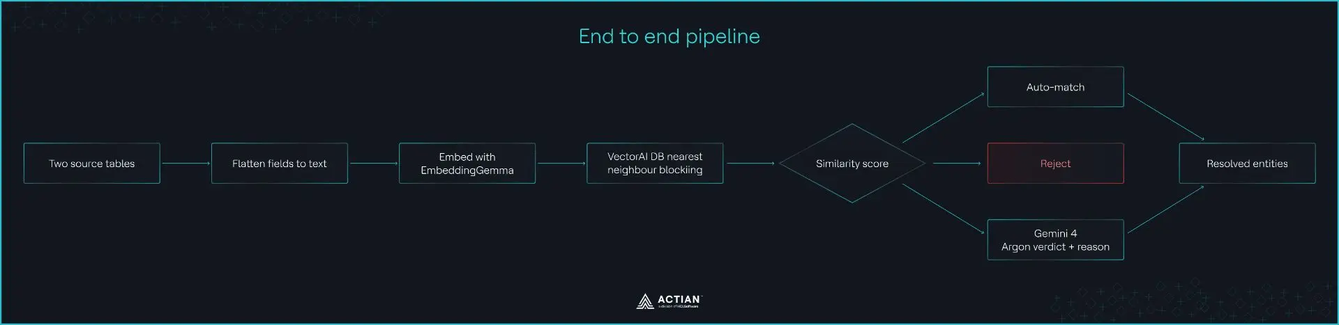
The pipeline. Records are embedded and blocked in VectorAI DB, and the similarity score routes each candidate pair to an auto-match, a rejection, or Argon.
The examples use Abt-Buy, a standard data matching benchmark from the Leipzig collection: 1,081 Abt products and 1,092 Buy products, with a gold file listing the 1,097 true matches. Comparing every Abt record with every Buy record would mean 1,081 × 1,092 = 1,180,452 pairs.
Step 1: Start VectorAI DB
Clone the companion repo and move into the project folder. Every command from here on runs in this folder:
git clone https://github.com/actian-devs/developer-content.git
cd developer-content/blog/entity-resolution-vectorai
The repo’s docker-compose.yml starts VectorAI DB. The ACTIAN_VECTORAI_ACCEPT_EULA=YES line accepts Actian’s license for you, so read it before you start the container:
services:
  vectorai:
    image: actian/vectorai:1.0.2
    container_name: vectorai
    ports:
      - "6573:6573" # REST
      - "6574:6574" # gRPC (Python SDK)
      - "6575:6575" # Local UI
    volumes:
      - ./vectorai_data:/var/lib/actian-vectorai
    environment:
      - ACTIAN_VECTORAI_ACCEPT_EULA=YES
    restart: unless-stopped
Start it:
docker compose up -d
docker ps
The container should show Up. The Python SDK talks to it over gRPC on port 6574.
The Community Edition‘s 5,000-vector cap covers the whole server, and deleted vectors kept counting against it until we restarted the container. The harness drops its own old collections; if it still reports the cap, run docker compose restart vectorai.
Step 2: Pull the Embedding Model
Install Ollama, then pull EmbeddingGemma, about 620 MB:
ollama pull embeddinggemmaOllama serves it on localhost:11434, and the harness calls it there. Nothing leaves your machine at this stage.
Step 3: Install Python Dependencies
The repo already includes pyproject.toml, shown below for reference. Its uv.lock pins the exact versions we ran, such as actian-vectorai-client 1.0.3 and google-genai 2.31.0:
[project]
name = "entity-resolution-vectorai"
version = "0.1.0"
description = "Entity resolution with VectorAI DB blocking and Gemini 4 Argon on the ambiguous band"
requires-python = ">=3.11,<3.14"
# uv run resolve.py reads this, creates .venv and installs these on first run
dependencies = [
    "actian-vectorai-client",  # VectorAI DB client (gRPC)
    "google-genai",            # Gemini API, for the Argon pass
    "pandas",
    "numpy",
    "pydantic",                # Argon's structured-output schema
    "requests",                # benchmark download
    "matplotlib",              # score-distribution chart
]

[project.optional-dependencies]
st = ["sentence-transformers"]   # in-process embedding models: uv sync --extra st, then --embed-backend sentence-transformers
Create the environment:
uv syncFrom here on, start each command with uv run; you don’t need to activate an environment.
Step 4: Load and Embed the Records
The source table goes into each point’s payload because Step 5 filters on it, so an Abt record is only ever compared with Buy records. Embedding is the slowest step on a CPU the harness caches the vectors, and reruns skip it. The code below is the core of three functions in the repo load() in er/data.py builds records, a list of (source, record_id, text) tuples with the Abt records first embed() is in er/embed.pyand the upsert is load_records() in er/block.py.
import numpy as np
import requests
from actian_vectorai import Distance, PointStruct, VectorAIClient, VectorParams

def to_text(row, fields):
    # "name: Sony Bravia 40in LCD TV | price: $899.99" (empty fields are skipped)
    return " | ".join(f"{f}: {row[f].strip()}" for f in fields if row[f].strip())

def embed(texts, model="embeddinggemma", url="http://localhost:11434", batch=64):
    out = []
    for i in range(0, len(texts), batch):
        r = requests.post(f"{url}/api/embed", json={"model": model, "input": texts[i:i + batch]}, timeout=600)
        r.raise_for_status()
        out.extend(r.json()["embeddings"])
    v = np.asarray(out, dtype=np.float32)
    return v / np.linalg.norm(v, axis=1, keepdims=True)   # unit length, so cosine score = dot product

vectors = embed([text for , , text in records])          # records: (source, record_id, text)

with VectorAIClient("localhost:6574") as db:
    if db.collections.exists("er_abt_buy"):   # start clean, so the step can be rerun
        db.collections.delete("er_abt_buy")
    db.collections.create("er_abt_buy", vectors_config=VectorParams(
        size=vectors.shape[1], distance=Distance.Cosine))
    points = [PointStruct(id=i, vector=v.tolist(), payload={"source": src, "record_id": rid, "text": t})
              for i, ((src, rid, t), v) in enumerate(zip(records, vectors))]
    for start in range(0, len(points), 500):   # upsert in batches
        db.points.upsert("er_abt_buy", points[start:start + 500])
Step 5: Block With VectorAI DB
The blocking query runs once per Abt record and asks for its K nearest Buy records, with a must filter on the source field in each point’s payload. Here the rule is that a match always links one Abt record to one Buy record, so the search should only return records from the other source. Blocking on pre-trained embeddings like this has been studied at scale: Zeakis et al. evaluated 12 language models on 17 entity resolution benchmarks, including how well their embeddings block. The code continues from Step 4 and is the core of neighbours() in er/block.py.
from actian_vectorai import Field, FilterBuilder, VectorAIClient

K = 10
TOTAL_RECORDS = len(records)   # Abt + Buy: a limit this high returns every Buy record
abt_ids = [rid for src, rid,  in records if src == "abt"]
abtvectors = vectors[:len(abt_ids)]   # records lists every Abt record first
other_source = FilterBuilder().must(Field("source").eq("buy")).build()

def search(db, vectors, limit):
    out = []
    for i in range(0, len(vectors), 100):   # search_batch takes up to 100 queries per call
        out += db.points.search_batch("er_abt_buy", [
            {"vector": v.tolist(), "limit": limit, "filter": other_source, "with_payload": True}
            for v in vectors[i:i + 100]])
    return out

ranked, todo, limit = {}, list(range(len(abt_ids))), K  10   # over-fetch, then keep the top K
with VectorAIClient("localhost:6574") as db:
    while todo:
        short = []
        for i, hits in zip(todo, search(db, abt_vectors[todo], limit)):
            ranked[abt_ids[i]] = sorted(((h.payload["record_id"], h.score) for h in hits),
                                        key=lambda x: -x[1])[:K]
            if len(hits) < K and limit < TOTAL_RECORDS:   # stop once the limit covers the table
                short.append(i)
        todo, limit = short, min(limit  4, TOTAL_RECORDS)   # retry any record still short
Over-fetch when you filter. We measured this on VectorAI DB 1.0.2 with the 1.0.3 Python client and all 2,173 Abt-Buy records in one collection. A search_batch call with limit=10 and the source = buy filter came back short for 1,075 of the 1,081 Abt records, with 3.9 results on average. An unfiltered search for 10 neighbors returned Abt records 75.5% of the time. So the filtered results looked like the Buy records among roughly the limit nearest records overall, not the 10 nearest Buy records. The VectorAI DB predicate filters guide says filters apply during the search, so treat this as what 1.0.2 did on our collection, not as documented behavior.
Raising hnsw_ef, the HNSW index’s search breadth, to 256 changed nothing. A payload index on source wasn’t an option: 1.0.2 rejects adding one to an existing collection (“dynamic index creation not yet implemented”), and the 1.0.3 Python client has no setting to declare one when the collection is created. Asking for 10 × K and keeping the top K fixed it: every record got its 10 candidates, and 99.95% of them match an exact brute-force search.
On customer or supplier data, the same must clause can carry the rules that rule a pair out completely, such as a different country or a person against a company. Should clauses can favor candidates that share a field, such as a postcode, without excluding the rest. Budget for the same over-fetch: on 1.0.2, the more records a filter excludes, the fewer of the nearest records pass it, so raise the limit until every record gets its K.
Read the reduction ratio and pair completeness together
Two numbers describe blocking, and either alone misleads:
- Reduction ratio is the share of all pairs that blocking removed: 1 − candidates / all pairs.
- Pair completeness is the share of true matches that survived blocking: true matches among the candidates / all true matches.
import pandas as pd

candidates = {(abt_id, buy_id): score for abt_id, hits in ranked.items() for buy_id, score in hits}
n_buy = len(records) - len(abt_ids)
gold = set(map(tuple, pd.read_csv("data/abt-buy/abt_buy_perfectMapping.csv").astype(str).values))
rr = 1 - len(candidates) / (len(abt_ids) * n_buy)
pc = len(gold & candidates.keys()) / len(gold)
The harness computes both in blocking_quality() in er/block.py. Every true match that blocking drops is lost for good, so pair completeness caps recall for the whole pipeline. We swept K:
| K | Candidate pairs | Reduction ratio | Pair completeness |
|---|---|---|---|
| 1 | 1,081 | 99.91% | 81.9% |
| 3 | 3,243 | 99.73% | 94.5% |
| 5 | 5,405 | 99.54% | 97.0% |
| 10 | 10,810 | 99.08% | 99.0% |
| 20 | 21,620 | 98.17% | 99.7% |
We kept K = 10. It removed 99.08% of the comparison space and kept 99.0% of the true matches. Going to K = 20 adds 0.7 points of pair completeness for twice the candidates. Read the two numbers as a trade before you trust either: every pair blocking drop is a comparison saved and possibly a match lost for good. Pick the smallest K whose pair completeness you can live with, because that number is the recall ceiling for every step after it.
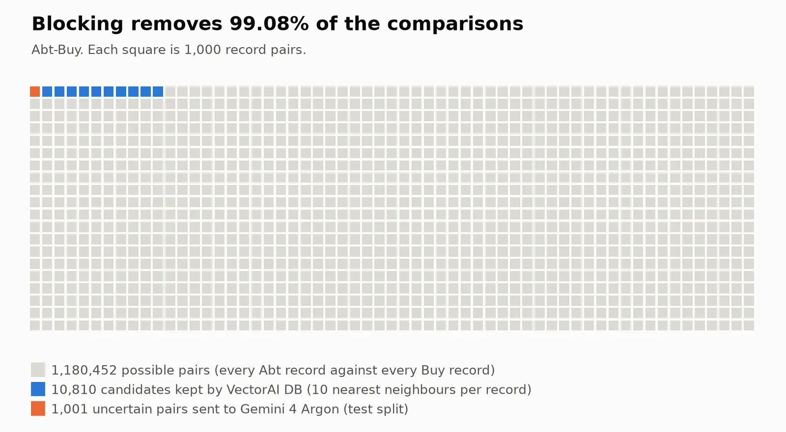
The comparison space on Abt-Buy: one square per 1,000 pairs. VectorAI DB kept 10,810 of the 1,180,452 possible pairs, and Argon read 1,001 of them.
Step 6: Score the Candidates and Set the Band
A single cutoff gets the close pairs wrong in both directions, so the pipeline splits candidates into three bands and hands only the middle one to Argon. The baseline is a best-match threshold: each Abt record’s nearest candidate is a match if its similarity clears one cutoff. Precision is the share of predicted matches that are real, recall is the share of real matches found, and F1 balances the two. On the Abt-Buy test split, the best cutoff was 0.562: precision 0.820, recall 0.806, F1 0.813. One global cutoff over all 10 candidates per record scored only 0.522.

Similarity of each Abt record’s nearest Buy candidate on the test split. All 136 false matches sit inside the band, between 0.56 and 0.84, mixed in with true matches, so no single cutoff can separate them.
Pick the band edges from the data
We held out 30% of the Abt records as a development split, set the cutoff and both edges from its score distribution, and report every result on the remaining 70%. The code below comes from er/bands.py, which also holds the helpers it uses: info maps each candidate to its rank and gap (rank_and_gap()), dev_best keeps each development record’s nearest candidate (best_match()), and best_cutoff is the baseline’s cutoff (best_threshold()). The edges work like this:
- Upper edge: The lowest score above which best matches reach 95% precision on the development split. Best matches above it are auto-matched.
- Lower edge: The highest score below which at most 5% of true matches fall, capped at the baseline’s cutoff so the pipeline never rejects a pair the baseline would accept. Pairs below it are rejected.
- Near-ties: A second- or third-ranked candidate that scores within 0.03 of its record’s best also enters the band. Nearest candidates alone cap recall at 82%, because 18% of true matches are not their record’s top candidate.
import numpy as np

def band_edges(cand, gold, target_precision, max_miss):
    pairs = sorted(cand.items(), key=lambda kv: kv[1], reverse=True)
    s = np.array([score for , score in pairs])
    y = np.array([p in gold for p,  in pairs], dtype=float)
    precision_above = np.cumsum(y) / np.arange(1, len(y) + 1)
    ok = np.where(precision_above >= target_precision)[0]
    upper = s[ok.max()] if len(ok) else s[0] + 1e-9   # nothing reaches the target: auto-match nothing
    missed_below = (y.sum() - np.cumsum(y)) / y.sum()   # share of matches scoring below each position
    lower = s[np.where(missed_below <= max_miss)[0].min()]
    return float(min(lower, upper)), float(upper)

def near_tie_band(cand, info, lower, upper, max_rank=3, max_gap=0.03):
    band = []
    for pair, score in cand.items():
        rank, gap = info[pair]   # rank among the record's candidates, distance below its best
        if score < lower:
            continue
        if (rank == 1 and score < upper) or (2 <= rank <= max_rank and gap <= max_gap):
            band.append(pair)
    return band

lower, upper = band_edges(dev_best, dev_gold, target_precision=0.95, max_miss=0.05)
lower = min(lower, best_cutoff)   # never reject a pair the baseline accepts
band = near_tie_band(test_candidates, info, lower, upper)
The edges landed at 0.562 and 0.841. The band held 1,001 of the 7,570 test candidates, 13.2%, and 206 of the baseline’s 279 errors sat inside it. If Argon decided every band pair correctly, recall could rise from 0.806 to 0.897. Measure that share on your own data before anything else: a single cutoff forces every close pair to one side, and only the errors that land in the band can be handed to a second pass. If most of them land elsewhere, no second pass will fix them.
What the threshold gets wrong
These pairs come from the band. Their vectors are close, and the right answer depends on a detail an embedding blurs. The table shows product names only. The harness embeds, and later sends to Argon, every field of each record: name, description, and price for Abt, and name, description, manufacturer, and price for Buy.
| Record A (Abt) | Record B (Buy) | Score | Truth | Baseline says |
|---|---|---|---|---|
| Sharp AQUOS 37′ Black LCD HDTV – LC37D64U | Sharp AQUOS LC37D44U 37′ LCD TV – LC37D44U | 0.832 | No match | Match |
| Sharp AQUOS 37′ Black LCD HDTV – LC37D64U | Sharp AQUOS LC-37D64U 37′ LCD TV | 0.814 | Match | No match (2nd candidate) |
| Omnimount Wall Speaker Mount – 20WLBK | OmniMount Stainless Steel Speaker Mount – 20.0 WALL-W | 0.830 | No match | Match |
| Omnimount Wall Speaker Mount – 20WLBK | OmniMount Universal Wall Speaker Mounting Kit – 20.0 WALL-B | 0.829 | Match | No match (2nd candidate) |
| Garmin Vehicle Adjustable Suction Cup Mount – 0101082303 | Garmin Vehicle Suction Cup mount | 0.832 | No match | Match |
The right Buy record is often the second candidate, just below a near-identical wrong one: the correct Sharp LC-37D64U scores 0.018 below the LC37D44U. Both clear any cutoff. The model number is the clearest difference, and the descriptions add others, such as a 10,000:1 against a 7500:1 contrast ratio. Here is the first pair as the embedding model and Argon see it:
Record A (Abt): name: Sharp AQUOS 37' Black LCD HDTV - LC37D64U | description: Sharp AQUOS 37' Black LCD HDTV - LC37D64U/ 1920 x 1080p Pixel Resolution/ Up To 60,000 Hours Lamp Life/ Built-In ATSC/QAM/NTSC Tuner/ 10,000:1 Dynamic Contrast Ratio/ 4ms Response Time/ 4-Wavelength Backlight System/ Black Finish

Record B (Buy): name: Sharp AQUOS LC37D44U 37' LCD TV - LC37D44U | description: Sharp AQUOS LC-37D44U - 37' Widescreen LCD HDTV - 7500:1 Dynamic Contrast Ratio - 6ms Response Time | manufacturer: Sharp
Step 7: Send the Band to Argon
Each band pair goes to Argon and comes back as a match or no-match with a one-sentence reason. The response is structured output, JSON that fits a schema, so you don’t parse anything by hand. A general model can do this step without training data: Peeters, Steiner and Bizer found that the best LLMs, given no or few examples, match pre-trained language models fine-tuned on thousands of labeled pairs. The prompt and schema below are the ones in the repo, fixed on the development split, and the code is the core of the Adjudicator class in er/adjudicate.py. This snippet calls the Gemini API directly with GEMINI_API_KEY; the harness can also reach the same model through OpenRouter.
import json
from google import genai
from google.genai import types
from pydantic import BaseModel

class Verdict(BaseModel):
    match: bool
    reason: str   # one sentence, logged for audit

PROMPT = """You are resolving product records from two catalogues.
Decide whether Record A and Record B describe the same product: same model, size, and variant.
Answer from the records only. Give a one-sentence reason.

Record A: {a}
Record B: {b}"""

client = genai.Client()   # reads GEMINI_API_KEY from the environment

def adjudicate(a_text: str, b_text: str) -> tuple[Verdict, int, int]:
    resp = client.models.generate_content(
        model="gemini-4-argon",
        contents=PROMPT.format(a=a_text, b=b_text),
        config=types.GenerateContentConfig(
            response_mime_type="application/json",
            response_schema=Verdict,
            temperature=0,
            thinking_config=types.ThinkingConfig(thinking_level="LOW"),
        ),
    )
    usage = resp.usage_metadata
    # thinking tokens are billed at the output rate, so count them with the visible answer
    out_tokens = (usage.candidates_token_count or 0) + (usage.thoughts_token_count or 0)
    return Verdict.model_validate_json(resp.text), usage.prompt_token_count or 0, out_tokens
Every verdict goes to a log with its reason, so when a merge is questioned later you can show why Argon made it. The loop skips pairs already in the log, so a rerun never pays twice; the harness adds retries for rate limits on top:
import os

text_of = {(src, rid): text for src, rid, text in records}

os.makedirs("results", exist_ok=True)
log_path = "results/argon_verdicts.jsonl"
done = set()
if os.path.exists(log_path):   # pairs already paid for on an earlier run
    with open(log_path) as f:
        done = {(r["abt"], r["buy"]) for r in map(json.loads, f)}

tokens_in = tokens_out = 0
with open(log_path, "a") as log:
    for abt_id, buy_id in band:
        if (abt_id, buy_id) in done:
            continue
        verdict, t_in, t_out = adjudicate(text_of["abt", abt_id], text_of["buy", buy_id])
        tokens_in += t_in
        tokens_out += t_out
        log.write(json.dumps({"abt": abt_id, "buy": buy_id, **verdict.model_dump()}) + "\n")
        log.flush()   # a crash mid-run keeps every verdict written so far
The runs in this article reached Argon through OpenRouter, which routes to Google’s endpoints and reports the exact charge per call. Thinking was set to LOW, because thinking tokens are billed and a match decision doesn’t need deep reasoning.
Set your key before you run the harness, in the environment and never in the code. The snippet above reads GEMINI_API_KEY the harness’s OpenRouter backend (–argon-backend openrouter) reads OPENROUTER_API_KEY:
# macOS or Linux
export OPENROUTER_API_KEY="<YOUR_OPENROUTER_API_KEY>"

# Windows (PowerShell)
$env:OPENROUTER_API_KEY="<YOUR_OPENROUTER_API_KEY>"
The harness also enforces a spending cap: –budget-usd adds up the exact cost of every call across all runs and stops before the cap.
What Argon decided
As above, the table shows names only; Argon read the full records. The Garmin row’s Buy description, for example, carries the part number 010-10723-03 that Argon cites.
| Record A (Abt) | Record B (Buy) | Truth | Argon | Argon’s reason |
|---|---|---|---|---|
| Sharp AQUOS 37′ Black LCD HDTV – LC37D64U | Sharp AQUOS LC37D44U 37′ LCD TV – LC37D44U | No match | No match | Different Sharp AQUOS 37-inch models, the LC37D64U and the LC37D44U, which also have different contrast ratios. |
| Sharp AQUOS 37′ Black LCD HDTV – LC37D64U | Sharp AQUOS LC-37D64U 37′ LCD TV | Match | Match | The same 37-inch Sharp AQUOS LCD HDTV with the same model number (LC37D64U / LC-37D64U) and 1920 x 1080 resolution. |
| Omnimount Wall Speaker Mount – 20WLBK | OmniMount Stainless Steel Speaker Mount – 20.0 WALL-W | No match | No match | Record A is the black variant (20WLBK, black finish); Record B is a different variant (20.0 WALL-W). |
| Omnimount Wall Speaker Mount – 20WLBK | OmniMount Universal Wall Speaker Mounting Kit – 20.0 WALL-B | Match | Match | The same black stainless steel mount rated to 20 lbs; 20WLBK and 20.0 WALL-B are the same model. |
| Garmin Vehicle Adjustable Suction Cup Mount – 0101082303 | Garmin Vehicle Suction Cup Mount | No match | No match | Different part numbers: 0101082303 against 010-10723-03. |
Argon got 960 of the 1,001 band pairs right, 95.9%, including every pair above that the threshold had wrong. Forty of its 41 mistakes were true matches it declined, and our reading of its logged reasons sorts them into three groups:
- One record too vague to confirm (19). Buy lists “LG 2.0 cu.ft. Over the Range Microwave Oven” with no model number or color, so Argon would not call it the same product as a specific model.
- A variant, color, or bundle difference (7). A black Canon PowerShot against the silver one, or an SD card sold with a card reader against the card alone. The benchmark counts these as matches; Argon does not.
- Different model numbers (14). Several look like labeling errors in the benchmark itself, such as the Weber Summit S-650 against the S-450 and Apple’s 500 GB Time Capsule against the 1 TB model.
The 41st mistake went the other way: Argon matched an LG French-door refrigerator listed at 25.0 cu. ft. with one listed at 24.7 cu. ft., reasoning that 24.7 is the exact capacity of the same model, and the benchmark says they differ.
The reasons show a model applying a stricter idea of “the same product” than the benchmark’s labels. They also show where the fix lies. A better prompt can’t supply a model number a record doesn’t have, and a wider band doesn’t help pairs Argon already sees. For the 19 vague pairs, the fix is records that say enough, and for the 14 model-number pairs it is checking the labels.
Step 8: Run the Full Pipeline
The full harness, with blocking, band selection, the Argon pass, and scoring against the gold labels, is in the companion repo. Versions are pinned:
| Component | Version |
|---|---|
| VectorAI DB | actian/vectorai:1.0.2 |
| Embedding model | EmbeddingGemma (embeddinggemma) through Ollama |
| Adjudicator | gemini-4-argon, run on 23 October 2026 through OpenRouter, thinking level LOW |
| Datasets | Abt-Buy and Amazon-Google, Leipzig benchmark collection, downloaded 19 October 2026 |
Run the whole pipeline on Abt-Buy:
uv run resolve.py --dataset abt-buy --argon-backend openrouter --workers 2 --budget-usd 10Swap in –dataset amazon-google for the second benchmark, or add –no-argon to run blocking and the threshold without any API calls.
The script prints every metric in this article for both approaches, plus the share of pairs sent to Argon and the cost. Trimmed output from the Abt-Buy run:
abt-buy: 1081 abt + 1092 buy records, 1097 true matches

Blocking (all records, hnsw_ef=256):
  K=1   candidates=  1,081  reduction ratio=0.9991  pair completeness=0.8186  returned/record: mean 1.0, min 1, short 0
  K=3   candidates=  3,243  reduction ratio=0.9973  pair completeness=0.9453  returned/record: mean 3.0, min 3, short 0
  K=5   candidates=  5,405  reduction ratio=0.9954  pair completeness=0.9699  returned/record: mean 5.0, min 5, short 0
  K=10  candidates= 10,810  reduction ratio=0.9908  pair completeness=0.9900  returned/record: mean 10.0, min 10, short 0
  K=20  candidates= 21,620  reduction ratio=0.9817  pair completeness=0.9973  returned/record: mean 20.0, min 20, short 0

Test split: 7,570 candidates, 767 true matches
  Global cutoff, all candidates (reference, 0.7672): P=0.5734 R=0.4785 F1=0.5217
  Best-match threshold (baseline, 0.5618): P=0.8196 R=0.8057 F1=0.8126
  Band [0.5618, 0.8405) + near-ties (rank <= 3, gap <= 0.03): 1,001 pairs (13.2% of candidates), holding 206/279 of the baseline's errors; recall ceiling 0.8970
  With Argon: P=0.9985 R=0.8449 F1=0.9153  (960/1001 band verdicts correct, $1.4081)
The Results, Measured
The Argon pass raised F1 by about 10 points on both benchmarks, from 0.813 to 0.915 on Abt-Buy and from 0.597 to 0.691 on Amazon-Google, while reading 13 to 14% of the candidate pairs. That is not a rounding error: on Abt-Buy it removed 135 of the 136 false matches the threshold accepted. Whether a lift is worth it on your data depends on what a wrong merge or a missed match costs you. A lift of a point or two would be hard to tell apart from moving the cutoff, and wouldn’t justify an API bill.
| Dataset | Reduction ratio | Pair completeness | F1, best-match threshold | F1, with Argon | Share sent to Argon | Cost per 1,000 records |
|---|---|---|---|---|---|---|
| Abt-Buy | 99.08% | 99.0% | 0.813 | 0.915 | 13.2% | $0.76 |
| Amazon-Google | 99.69% | 94.1% | 0.597 | 0.691 | 14.0% | $0.58 |
Precision and recall show where the lift came from. On Abt-Buy, precision rose from 0.820 to 0.998 and recall from 0.806 to 0.845. Inside the band, Argon rejected 135 of the 136 false matches the threshold had accepted, and it accepted 59 true matches that were a record’s second- or third-best candidate, which a best-match threshold can never pick. Recall stopped short of the band’s 0.897 ceiling because Argon declined pairs where one record was too vague, or where the products differed in variant, color, or bundle.
Amazon-Google is harder: its software titles vary in edition, version, and packaging, and blocking kept 94.1% of true matches. Precision rose from 0.581 to 0.684 and recall from 0.614 to 0.698, and Argon was right on 76.4% of the band. Most of its 316 errors (290) were matches to the gold file rejects. In a random sample of 12, seven share an explicit model number, part number, or version with the matched listing, such as Netgear’s VPN01L, which points to gaps in the gold labels. All scores here still use the gold file as published.
Cost. At OpenRouter’s exact per-call charges, including thinking tokens, the 1,001 Abt-Buy calls cost $1.41, and the 1,338 Amazon-Google calls cost $2.42. Per 1,000 records in each test split, counting the test-split records from the first table plus the whole second table (1,849 records for Abt-Buy, 4,181 for Amazon-Google), that is $0.76 and $0.58. Argon’s list price doubles on 1 December 2026, according to Google’s Gemini API pricing page, which would roughly double these figures. For a managed reference point, AWS Entity Resolution charges $0.25 per 1,000 records processed for rule-based or ML matching, on every record rather than on a band.
Latency. On a CPU-only laptop with 8 GB of RAM, embedding the 2,173 Abt-Buy records took 771 seconds, and blocking took 35 seconds. The Argon calls took 54 minutes for Abt-Buy and 88 minutes for Amazon-Google, with 2 requests in parallel; at 8 parallel requests, our calls came back with 429 rate-limit errors. Embedding is a one-time cost: the harness caches the vectors, so reruns start at blocking.
Against the literature. Li et al. report that Ditto, a matcher fine-tuned on labeled pairs, reaches an F1 of 89.33 on Abt-Buy and 75.58 on Amazon-Google (0.893 and 0.756 on the scale used here) on the ER-Magellan versions of these benchmarks. Ditto was scored on a pre-selected set of labeled pairs, while our numbers come from resolving the full tables after blocking, so treat its scores as a reference point. Our pipeline needs no training data, and its recall is capped by what blocking keeps and by which candidates reach the band.
Why it Runs on Your Own Infrastructure
Resolution data is customers, patients, and counterparties- records that often cannot leave a regulated boundary. Here, VectorAI DB and the embedding model run on your own machines, so the embeddings, the blocking, and the resolved entities stay inside your network. Only the Argon call sends data out: the band, 13.2% of candidate pairs, two records at a time. For regulated data, pick one of two paths:
- De-identify the band. Strip or mask names, emails, and account numbers, and send only the fields that decide the match, if your policy allows any data to leave.
- Keep the second pass local. If no field may leave, swap adjudicate() for a call to a model you host. The code structure stays the same. We did not measure a local model in this run, so expect different accuracy and cost numbers.
When the Collaboration is Worth it, and When it is Not
This split takes a side in a live argument about LLMs in entity resolution. Jeff Jonas, Senzing’s founder, writes that he is often asked why not just use an LLM for entity resolution, and answers that it is “not a good idea.” He points to Clair Sullivan’s comparison of Claude Opus 4.8 against Senzing’s engine, where the LLM was far slower and costlier, and to deterministic outcomes and explainability. The pipeline here agrees on scale and keeps the LLM away from almost every pair; VectorAI DB and the threshold decide 87% of the candidates, and Argon reads only the band where the threshold is unreliable. It answers part of the explainability point too, since every verdict is logged with its reason. It doesn’t make Argon deterministic, but a rerun replays the logged verdicts instead of asking again.
Run the Argon pass when two things hold on your data: the band holds most of the threshold’s errors, and Argon decides band pairs at least 10 points more accurately than the threshold does. Both held on both benchmarks, and each time the pass bought about 10 F1 points for under $1 per 1,000 records.
| Dataset | Threshold’s errors inside the band | Threshold right on band pairs | Argon right on band pairs | F1 gain | Cost per 1,000 records |
|---|---|---|---|---|---|
| Abt-Buy | 206 of 279 (74%) | 79.4% | 95.9% | +10.3 | $0.76 |
| Amazon-Google | 500 of 697 (72%) | 62.6% | 76.4% | +9.4 | $0.58 |
Argon’s lead on band pairs was 16.5 points on Abt-Buy and 13.8 on Amazon-Google. To find where that lead stops buying F1, we reran the band at half and twice its width on both datasets. Every verdict came from the same log, so each row shows what the extra slice of the band added:
| Dataset | Band width | Pairs sent to Argon | F1 with Argon | Argon cost | Argon’s lead on the pairs added |
|---|---|---|---|---|---|
| Abt-Buy | 0.5× | 803 | 0.901 | $1.13 | (base) |
| Abt-Buy | 1× | 1,001 | 0.915 | $1.41 | +12.1 points on 198 pairs |
| Abt-Buy | 2× | 1,079 | 0.916 | $1.53 | +1.3 points on 78 pairs |
| Amazon-Google | 0.5× | 1,269 | 0.6905 | $2.32 | (base) |
| Amazon-Google | 1× | 1,338 | 0.6909 | $2.42 | +1.4 points on 69 pairs |
| Amazon-Google | 2× | 1,348 | 0.6924 | $2.44 | +20 points on 10 pairs |
The slices where Argon beat the threshold clearly paid. On Abt-Buy, the half-to-full slice, a 12.1-point lead, added 1.5 F1 points for $0.28. On Amazon-Google, the last 10 pairs, a 20-point lead, added 0.15 points for $0.02. The slices where it led by about a point added under a tenth of a point each: the next 78 Abt-Buy pairs added 0.07 for $0.12, and the half-to-full slice on Amazon-Google added 0.04 for $0.09. So the extra spend stopped buying F1 somewhere between a 1-point and a 12-point lead. Two datasets can’t place that line more exactly, so treat the 10-point bar as a rule of thumb that sits inside the gap.
The pass stops paying in three cases:
- The threshold is already right on the band. If your threshold-based band pairs nearly as well as Argon does, the pass spends money confirming what the threshold already knew.
- The errors sit outside the band. If blocking drops true matches, or they rank too deep to count as near-ties, no second stage sees them. On Amazon-Google that capped recall at 0.727 before Argon read a single pair.
- The band is too wide. Doubling the band’s width on Abt-Buy sent 78 more pairs to Argon (1,079 instead of 1,001) and cost $0.12 more at OpenRouter’s measured charges, but only one more of the threshold’s errors fell inside it. F1 moved from 0.9153 to 0.9160, under a tenth of a point. Set the edges from your data, then leave them.
To check your own data, label about 200 band pairs by hand, then compare how often the threshold and Argon get them right. That sample costs about 30 cents in Argon calls at the rates measured here, and it tells you whether the full pass will pay before you run it.
Conclusion
The pipeline in this article got the Sharp TVs from the opening right. The threshold picked the LC37D44U because its vector scored higher; Argon read both records, matched the LC37D64U by its model number, and logged why. Across the Abt-Buy test split, that second pass lifted F1 from 0.813 to 0.915 for $0.76 per 1,000 records.
That result comes from three decisions working together:
- Block with a filtered nearest-neighbor search in VectorAI DB, so 99% of the comparison space disappears while 99% of the true matches stay.
- Set the band edges from labeled data, so only the uncertain 13.2% of candidates costs money.
- Send just that band to a model that can read a part number.
VectorAI DB and the embedding model run on your own hardware, so everything except the band stays inside your network.
The same harness runs on your own tables. Point the loader at your customer, supplier, or product records, put your exclusion rules in the blocking filter’s must clause, and run it on VectorAI DB Community Edition. Pull the image to start:
docker pull actian/vectorai:latest
Stay connected
Data insights delivered to you.
(i.e. sales@..., support@...)
