How Actian Vector Helps You Eliminate OLAP Cubes


Actian Vector was renamed to Actian Analytics Engine in 2026.
OLAP (OnLine Analytical Processing) Cubes are used extensively today because many database platforms can’t analyze large volumes of data quickly. This is because most database software does not fully leverage computing power and memory to deliver optimal performance. Some of the symptoms of this are:
- Large queries end up hogging server resources.
- Response becomes slower as data size and the number of users increases.
- Supporting concurrent queries becomes difficult or impossible.
- Additional aggregated/materialized tables, indices and sometimes even individual data marts fail to deliver the required performance and concurrency.
OLAP Cube stores were created to solve a BI user’s need to quickly aggregate, slice and dice large amounts of data for a set of pre-determined questions. Now we’ll look at how we can use Actian Vector, our high-speed columnar analytics database, to eliminate the use of OLAP Cubes.
What are the Downsides of Using OLAP Cube Stores?
- Additional investment in hardware/software and ongoing maintenance costs.
- Completely new skills in Multi-Dimensional Expressions (MDX) are required to query the OLAP Cubes.
- Imposes a strict schema (star or snowflake), while some of the newer generation Cube stores support 3NF tables (or ROLAP models). But the best performance is always delivered by having a star schema.
- They limit ad-hoc query freedom. A lot of thought needs to go into designing the OLAP Cube. Once it is built, only the rows and columns included will be available for querying. Often, a new Cube is required for every new query.
- Adds a significant amount of processing time and creates new bottlenecks to the BI life cycle. The BI user would have to pay heavily in lost time if the OLAP Cube was built incorrectly. Data freshness is compromised as data has to move from operational systems to the data warehouse to the OLAP Cube and then to BI tools.
Looking Under the Hood
Let’s have a look at what you give up with an OLAP Cube. Here’s a simple example where the raw data in the underlying relational database looks as follows:
| Sale _date | Year | month | decade | city _id | city _name | state | Region _id | Region _name | Product _id | Product _name | Sales _Amount |
| 1/1/1990 | 1990 | January | 1990-2000 | 1 | Palo alto | CA | 1 | US-West | 1 | Bolts | 20 |
| 1/2/1990 | 1990 | January | 1990-2000 | 1 | Palo alto | CA | 1 | US-West | 1 | Bolts | 23 |
| 1/3/1990 | 1990 | January | 1990-2000 | 1 | Palo alto | CA | 1 | US-West | 1 | Bolts | 15 |
| 1/1/1993 | 1993 | January | 1990-2000 | 1 | Palo alto | CA | 1 | US-West | 2 | hammer | 14 |
| 5/1/1993 | 1994 | May | 1990-2000 | 2 | La Jolla | CA | 2 | US-West | 3 | screws | 60 |
| 1/1/2003 | 2003 | January | 2000-2010 | 3 | Dallas | TX | 1 | US-South | 1 | Bolts | 12 |
| 5/1/1993 | 1993 | May | 2000-2010 | 4 | Atlanta | GA | 2 | US-South | 3 | Screws | 34 |
| 10/1/2004 | 2004 | October | 2000-2010 | 5 | New York | NY | 1 | US-east | 1 | Bolts | 35 |
| 10/2/2004 | 2004 | November | 2000-2010 | 6 | Boston | MA | 1 | US-East | 1 | Bolts | 37 |
| 10/3/2004 | 2004 | December | 2000-2010 | 1 | Palo Alto | CA | 1 | US-West | 1 | Bolts | 39 |
| 10/4/2004 | 2004 | January | 2000-2010 | 1 | Palo Alto | CA | 1 | US-West | 1 | Bolts | 42 |
| 10/5/2004 | 2004 | February | 2000-2010 | 7 | Madison | WI | 1 | US-central | 1 | Bolts | 44 |
| 10/6/2004 | 2004 | March | 2000-2010 | 8 | Chicago | IL | 1 | US-central | 2 | hammer | 46 |
| 4/1/2011 | 2011 | April | 2010-2020 | 9 | Salt Lake City | UT | 2 | US-West | 3 | screws | 49 |
| 5/2/2012 | 2012 | May | 2010-2020 | 1 | Palo Alto | CA | 2 | US-West | 1 | Bolts | 51 |
| 6/3/2013 | 2013 | June | 2010-2020 | 2 | La Jolla | CA | 2 | US-West | 3 | Screws | 53 |
| 7/4/2014 | 2014 | July | 2010-2020 | 10 | Jersey City | NJ | 2 | US-East | 1 | Bolts | 56 |
If a user is interested in creating a simple OLAP Cube for sales from the data above and the metrics of interest aggregated sales_amounts for each decade, year, by product and region, the OLAP Cube would have the following data in it:
| Decade | Year | Region_name | Product_name | Sales_Amt | Avg_Price |
| 1990-2000 | 1994 | US-West | Screws | $60.00 | $19.33 |
| 1990-2000 | 1993 | US-South | Screws | $34.00 | $14.00 |
| 1990-2000 | 2003 | US-South | Bolts | $12.00 | $60.00 |
| 2000-2010 | 2004 | US-central | Bolts | $44.00 | $34.00 |
| 2000-2010 | 2004 | US-Central | Hammer | $46.00 | $12.00 |
| 2000-2010 | 2004 | US-east | Bolts | $72.00 | $44.00 |
| 2000-2010 | 2004 | US-West | Bolts | $81.00 | $46.00 |
| 2000-2010 | 2011 | US-West | Screws | $49.00 | $36.00 |
| 2010-2020 | 2012 | US-West | Bolts | $51.00 | $40.50 |
| 2010-2020 | 2013 | US-West | screws | $53.00 | $49.00 |
| 2010-2020 | 2014 | US-east | Bolts | $56.00 | $51.00 |
| 2010-2020 | 1994 | US-West | Screws | $60.00 | $53.00 |
The data is aggregated by Decade, Year, Region_name, Product_name. The transactional level detail is lost. For this reason, some of the more mature OLAP Cube stores offer a drill-through feature allowing the user a look at the detailed data. However, the performance could degrade if the amount of data behind the aggregation is large.
A typical MDX query to get this data from the cube would look like this based on what the user would like to see on rows and columns and data points.
WITH
MEMBER[measures].[avg price] AS
'[measures].[sales_amt] / [measures].[sales_num]'
SELECT
{[measures].[sales_sum],[measures].[avg price]} ON COLUMNS,
{[product].members, [year].members} ON ROWS
FROM SALES_CUBE
The Avg_price is a calculated measure. Note that calculated measures can be specified in the OLAP Cube definition or can be defined in the MDX query. One of the benefits of calculated measures defined in OLAP Cubes is that if the query was changed to have a filter or an additional dimension was added the calculated measure would automatically get recalculated with the new parameters.
And so, the OLAP Cube ends up being a partial fix to a problem – that row-oriented relational databases simply aren’t fast enough for analytic queries. What would your OLAP users ask for if they could have whatever they want? What we hear from users are these requirements:
- OLAP-like speed or better with full ad hoc query support
- The ability to use any data model they want
- All their favorite BI tools
- The most current data available
- Access to full detail data in the same query, and without trading away any performance
Seem impossible? It isn’t. Actian Vector can deliver all this and more. How is that possible? Read on!
Replacing OLAP Cubes With Vector
Actian Vector is uniquely positioned to replace OLAP Cubes. We built it from the ground up with a number of optimizations to dramatically increase the performance of analytic queries. Here’s a quick summary of what we’ve built:
- Vector Processing: Vectorization takes parallelization to the next level by sending a single instruction to multiple data points delivering near real-time response.
- Columnar Storage: Columnar greatly reduces IO by only loading the columns required in a query into memory as opposed to loading all the columns into memory and then picking the required columns required to satisfy the query.
- Optimized In-Memory: Advanced use of processor cache and main memory, and in-memory compression and decompression speed up the process.
- Flexibility: Vector works with any data-model – star, snowflake, 3NF and de-normalized eliminating the need to create any type of materialization of data. Since the BI user is working off of the source of data, query freedom is not lost.
- Functional Richness: Advanced OLAP/Windows functions empower the user to ask a wide array of sophisticated questions.
Moving From Cubes to Actian Vector
To migrate BI reports from OLAP Cubes, it is important to understand the Cube features that need to be migrated. These include:
- OLAP Cube Model – Understand the data model of the Cube itself and map it back to the RDBMS data model.
- MDX queries, calculated measures, and filters being used.
- KPIs – Key Performance Indicators.
- What-if analysis for different scenarios.
OLAP Cube Model
Examine the OLAP Cube and identify what sort of data model it relies on: ROLAP, HOLAP or MOLAP. ROLAP models rely on third-normal-form (3NF) data-models where the data is highly normalized. Typically, there is a performance penalty when using ROLAP models in Cubes.
HOLAP is a hybrid model where a combination of star or snow-flake models, de-normalized and 3NF is used. This also has performance penalties.
MOLAP is the most desired underlying model where a star or snow-flake data model is used and delivers the best performance. Typically, in a BI lifecycle, the source data is in 3NF and it must go through a long transformation process to get converted to a star schema model. The penalty is paid up-front to gain better performance later.
The following factors need to be examined, if a query is used at the data source:
- Dimensions: How is this arrived at in the Cube. Specially for ROLAP and HOLAP models.
- Measures: Both calculated and normal measures.
- Facts: Is it one single table, a combination of tables?
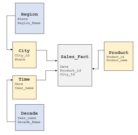
It is important to examine the above factors to gain an understanding of the underlying RDBMS model to see where these elements can be obtained. Typically, data warehouses have star or snow-flake models implemented but some data warehouses tend to have a highly normalized model. For the Cube above, a typical snow-flake model would look like follows:

Converting MDX Queries to SQL
Examine the MDX query and identify the following elements from the OLAP Cube and MDX query. Refer to a basic MDX tutorial if you need to. Here’s what you’ll need to know:
- Dimensions
- Measures
- Calculated Measures
- Slices of data or Filters (Example: If the user wanted to know the sales for only “Bolts” or only for the month of January.)
Taking the MDX query from the prior section as an example:
WITH
MEMBER[measures].[avg price] AS
'[measures].[sales_amt] / [measures].[sales_num]'
SELECT
{[measures].[sales_sum],[measures].[avg price]} ON COLUMNS,
{[product].members, [year].members} ON ROWS
FROM SALES_CUBE
Where:
- Avg price is a calculated measure
- Sales_amt is a measure that is defined in the cube
- [product].members is the product Dimension
- [Year].members is the year Dimension
Now you want to convert the MDX queries to SQL Queries based on the model above. The MDX query can be rewritten in SQL as below:
Select year_name, product_name, sum(sales_amt) as sales, avg(sales_amt) as avg_sales
from Sales                FT
join Time_Dimension        TD       on FT.date = TD.date
join Month_Dimension    MD     on month(TD.date) = MD.month
join Year_Dimension         YD       on year(date) = YD.year
join City_Dimension          RD       on FT.city_id = RD.city_id
join State_Dimension   SD on FT.state_id= RD.state_id
join Product PD on FT.product_id = PD.Product_id
group by year_name, product_name
or, simplify the query even more by removing the dimension tables if they were introduced only to build the Cube:
Select
date_part(year, sale_date) as year_name, product_name,
sum(sales_amt) as sales ,
avg(sales_amt). as avg_sales
from Sales FT
join Product PD on FT.product_id = PD.Product_id
group by decade,year_name, region_name, product_name
Note: It is not being implied that joins to other tables can be completely eliminated. Only tables that were introduced simply to adhere to the strict star/snow-flake schema can be eliminated.
If the BI tool does not provide window analytic functions refer to the analytical functions an window functions provided by Vector so it can be executed in-database.
If the user would like to drill down into a specific set of rows then the aggregation can be removed and the query can be executed in-database. As an example, if the user is interested in drilling into January 1993 sales figures for product Bolts, they could use the following SQL query:
Select
Date_part(year, sale_date) as year_name,
product_name, sales_amt as sales
from Sales    FT
join Product PD on FT.product_id = PD.Product_id
where Product_name = “Bolts”
and Date_part(year, sale_date) = “1993”
and Date_part(month, sale_date)  = “January”
Key Performance Indicators
In business terminology, a Key Performance Indicator (KPI) is a quantifiable measurement for gauging business success.
A simple KPI object is composed of: basic information, the goal, the actual value achieved, a status value, a trend value, and a folder where the KPI is viewed. Basic information includes the name and description of the KPI. In a Microsoft SQL Server Analysis Services Cube, the goal is an MDX expression that evaluates to a number. The actual value is an MDX expression that evaluates to a number. The status and trend value are MDX expressions that evaluate to a number. The folder is a suggested location for the KPI to be presented to the client.
While some OLAP cube stores do provide elegant and easy to use interfaces to store and implement KPIs and actions, these can easily be implemented by using a combination of more mainstream database features and application code.
What-if Analysis for Different Scenarios
What-if analysis capabilities are provided by some Cube stores with easy-to-use interfaces. This can also be implemented using database features and application code with some effort.
This type of analysis requires storing various scenarios and analyzing the impact of the current state of business against these different scenarios. This is commonly used in financial services/ trading businesses to constantly assess the risk and impact of trading.
A detailed analysis of requirements would be required and a bit out of scope for this blog post.
Summary
For OLAP users looking to simplify the BI life cycle, the Actian Vector analytics database provides a viable alternative to OLAP Cubes with its ground-breaking technology, superior performance and in-database analytic capabilities. The benefit of migrating is reduced costs and a better BI user experience by through query freedom.
Don’t simply take my word for it. Try it for yourself. We’ve prepared a guide and evaluation copy of Vector, along with all the supporting materials you’ll need to test Vector in about an hour. You can ask our active Vector community questions here.
Stay connected
Data insights delivered to you.
(i.e. sales@..., support@...)